Indexing Methods for Vector Retrieval
Advanced Vector Indexing Techniques for RAG
Watch the video
ChatGPT is pretty useful, but you can’t build a product out of it.
I have been talking about RAG for many videos now, and it’s not for nothing. As we’ve discussed in our book and course, retrieving documents or useful text is necessary for all LLM-based products.
You need to give additional information to your LLM if you want it to be really useful. Which means being more than just a Google assistant. It needs to have up-to-date context and relevant information to share with your user. Basically, you want your own LLM but without the cost of training one. This is why RAG exists.
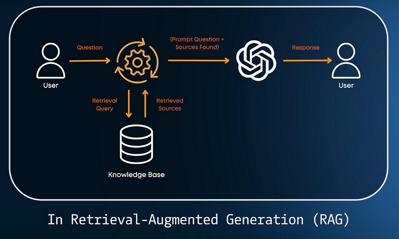
But what if your database is immense, or if there’s a massive chunk of information to compare? How do we ensure the “retrieval” part of the pipeline doesn’t slow us down?
To start, it’s important to know that when we retrieve information, we use a process called indexing. So, we have all our information stored in a database, and then we want to “index” it as efficiently as possible for future retrieval. Let’s see how we do that.
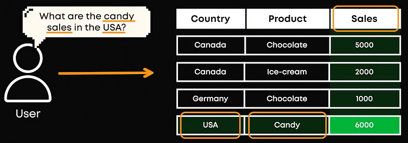
First, in normal databases or search queries, data is stored as rows, with columns providing more information about the document, such as metadata about the document; a date, authors, etc.. Using a query from a user, which is usually a question, we used to find exact or very similar matches. This has all changed with the LLM revolution. Instead of just finding precise matches, we use a vector database. Our vector database is basically all the database that we’ve fed into our LLM to retrieve its own understanding of it, which are our embeddings. These embeddings are just huge lists of numbers that are attached to the general meaning of each chunk of text from our database. Then, for each new query, we can feed it to our embedding system and use this list of numbers to compare it manually to all our database embeddings or vectors and retrieve the most similar ones. In short, in a vector database, we use the content itself (semantic search) to get similar content.
But we still have the volume problem. What happens if we have millions and millions of vectors? Do we still compare each of them in our database to our query vector? Not really! This is where we need a good vector index.
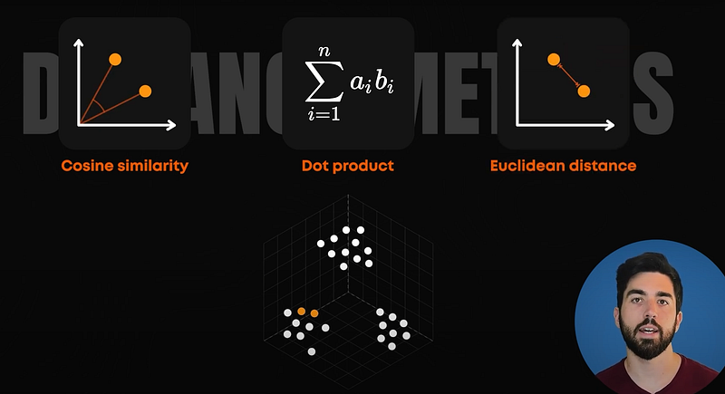
So what exactly is a vector index? It’s a data structure that searches and retrieves a vector embedding from a large dataset of objects. It needs to be both fast and accurate. As we’ve seen, an embedding is when an object is converted into a list of numbers. Each similar embedding is placed close to one another in the vector space. How do we know two embeddings are similar? We use distance metrics such as cosine similarity, dot product, or Euclidean distance to measure the distance and place the closer ones together. They are basically all ways of comparing the numbers in large lists together, and it gives us a number measuring that.
There are various methods to create vector indexes. Let’s look at some of the popular methods in detail. The easiest method is the Flat Index. Here, we convert the text into a vector embedding and store it as it is. We use a query to search it and get back the most similar information. The advantage is that it is highly accurate. Still, the disadvantage is that it makes searching very slow. You need to compare your query embedding with all your data.
The next type of indexing is Locality Sensitive Hashing (LSH) indexes. In this approach, vectors are grouped into buckets based on similarity, using specialized locality-sensitive hash functions. When a query vector is introduced, it is hashed using the same functions to identify the most similar bucket. Only the vectors within this bucket are then searched to find a match. It would be like a library where books are all categorized by fiction and genre. If you are looking for a specific book, you only need to look into its genre category instead of the whole library. You can then order it by last name, and you can find everything in a few seconds! This method ensures that similar items are grouped, making the retrieval process efficient and precise.
Another type of indexing is called the Inverted File Index. This is similar to LSH we just saw, but we use clustering to group vectors instead of hashing to create buckets. We take a centroid and compute the clusters. So we calculate all embeddings of our dataset and then group all of them using automatic algorithms that split our embeddings into dense groups based on resemblances. In our library example, comedy books might all be put together because of the laughs or other similar traits.
One problem with this method is that when a query lies at the boundary of multiple clusters, we tend to search all of them. An improved version is called Inverted File Product Quantization (IVFPQ). In IVFPQ, each vector within a cluster is further broken down into smaller sub-vectors, and these sub-vectors are encoded into bits, a process called Product Quantization, which really speeds up the comparison process. We then compare these smaller encoded bits instead of the original embeddings for more efficiency.

Finally, we have the Hierarchical Navigable Small Worlds (HNSW) index. It’s the most popular indexing method because it is fast and accurate, narrowing down the search area to make it easier to find what you need. How?
- We first need to build a Graph: You start with an empty graph that looks like this. When adding a document, you start at the top layer and navigate down, connecting to similar items at each layer. Each node is linked to its nearest neighbors, creating a multi-layered structure.

- Then, you search: When searching for a vector, you again begin at the top layer. You find the nearest neighbour and move down through its nearest neighbours. This continues layer by layer until you reach the bottom layer, where you find the very few most similar vectors.
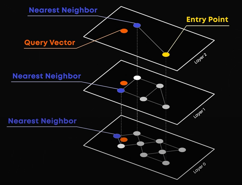
This process eliminates the vast majority of the data by going down the layers through broadly similar vectors in a step-wise fashion.
We now know what a good Index looks like. Let’s recap where it all fits together.
All your text, or data from your database, is split into small parts. We call these text parts our nodes. They are essentially individual segments or units of the original data, text chunks in our simple case here. These nodes are then converted into embeddings, numerical representations of the text, and stored in a vector index database. When your user asks a question, which is our query, it is converted into a vector embedding. Using the indexing method, the database searches for and returns the top results that match the query.
This is a basic setup, and there’s a lot you can do to enhance it. A first quick improvement would be to use prompting techniques to add context to the user question and help your retrieval system find the most relevant information possible, as some questions might lack a lot of detail and be quite broad, ending in disconnected embeddings versus what you are looking for.
Then, you can also implement other types of search methods with keywords or hybrid search to further improve the system and help your Indexing retrieve the desired information. There are also other new indexing methods like Multi-Scale Tree Graph (MSTG) you can look into. We cover all this in-depth in the course lessons and our book, which are all linked below if you watch this video from YouTube.
In any case, the use of vector indexes in RAG systems makes the retrieval of relevant information fast, accurate, and scalable. By converting text into vector embeddings and storing them in a structured vector index database, the system can quickly and efficiently find semantically similar content. In short: advanced indexing methods, such as HNSW, LSH, Product Quantization, or MSTG, reduce the search space and ensure the high relevance of the retrieved information.
This can all be done with great vector database platforms like ChromaDB or Pinecone using LlamaIndex, as we see in the course.
I hope you understand a bit more about what happens behind the scenes of indexing and why it’s important to implement one.

